Tutorial

This tutorial is presented for Windows. You may also run it on Linux or Mac OS, using *.sh files instead of *.bat files, and possibly python3 instead of python. We will go through the process of converting the IEEE 123-bus test system through CIM to both GridLAB-D and OpenDSS, comparing power flow solutions in both solvers. Then we will add houses and solar generation to the model, so we can impute feeder measurements from GridLAB-D simulations with weather data from Austin, TX.

Configuration Files

CIMHub uses two files to configure the Blazegraph database engine and the Java program, which exports models from CIM. These come properly configured for executing the tutorial on Windows, but in other scenarios you might have to make changes.

The Windows/tutorial cimhubjar.json is shown below.

• Line 2 specifies the TCP/IP port number 9999 and the Blazegraph namespace, which contains blazegraph for the recommended installation of v2.1.6

• Line 3 is the CIM namespace, which should not be changed.

• Line 4 may be required when using a restrictive proxy server, as at PNNL.

{
  "blazegraph_url": "http://localhost:9999/blazegraph/namespace/kb/sparql",
  "cim_ns": "<http://iec.ch/TC57/CIM100#",
  "use_proxy": true,
  "CIMHUB_PATH": "../releases/cimhub-1.1.0.jar",
  "CIMHUB_PROG": "gov.pnnl.gridappsd.cimhub.CIMImporter"
}

A sample Linux cimhubdocker.json is shown below. This is configured to use Blazegraph in Docker, with changes in Line 2:

• The port is 8889 from outside the Docker

• The namespace for v2.1.5 defaults to bigdata instead of blazegraph

{
  "blazegraph_url": "http://localhost:8889/bigdata/namespace/kb/sparql",
  "cim_ns": "<http://iec.ch/TC57/CIM100#",
  "use_proxy": true,
  "CIMHUB_PATH": "../releases/cimhub-1.1.0.jar",
  "CIMHUB_PROG": "gov.pnnl.gridappsd.cimhub.CIMImporter"
}

IEEE 123-Bus Base Case

In this first step, we run power flow in OpenDSS from a local copy of the IEEE test case and export the CIM XML. This XML file is uploaded to Blazegraph and then we export OpenDSS and GridLAB-D models from CIM. Power flow solutions from these two exported models are compared to the first one. At the end of this step, the CIM XML remains in Blazegraph.

• From a command prompt in c:\blazegraph, invoke go.bat. This starts the database engine. Leave this command prompt open, and don’t worry about any Java exceptions that are caught. When done with the tutorial, you can use Ctrl-C to stop the database engine, then close the command prompt.

• Open a second command prompt, navigate to ./tutorial in the CIMHub repository, and invoke python base123.py

• If everything goes well, you should see log messages and tabular output, completed within 10-20 seconds. Disregard any warnings about files or paths not found; they are from scripted removal of output directories to make a fresh start. The messages and outputs will be discussed below.

The Python script base123.py is shown below. As a roadmap to its contents:

• Lines 12-21 configure CIMHub for the operating system, choosing the jar version of Blazegraph for Windows and the docker version of Blazegraph for Linux or Mac OS. You may edit these lines, e.g., to use the jar on Linux.

• Lines 30-39 define the cases to run. There is just one for this tutorial, but there can be an array of them. Each case contains the following elements:

  • dssname is the root file name of the original OpenDSS base case

  • root is used to generate file names for converted files

  • mRID is a UUID4 to make the test case feeder unique. For a new test case, generate a random new mRID with this Python script import uuid;idNew=uuid.uuid4();print(str(idNew).upper())

  • substation is the name of a CIM substation to serve the feeder; the value does not affect power flow results

  • subregion is the name of a CIM subregion containing the CIM substation; the value does not affect power flow results

  • region is the name of a CIM region containing the CIM subregion; the value does not affect power flow results

  • glmvsrc is the substation source line-to-neutral voltage for GridLAB-D

  • bases is an array of voltage bases to use for interpretation of the voltage outputs. Specify line-to-line voltages, in ascending order, leaving out 208 and 480.

  • export_options is a string of command-line options to the CIMImporter Java program. -e=carson keeps the OpenDSS line constants model compatible with GridLAB-D’s. -l=1.0 scales the load to equal peak or nominal load. -p=1.0 specifies the load to be all constant power. (Use the -i and -z options to have constant current and constant impedance components of the load.)

  • skip_gld specify as True when you know that GridLAB-D won’t support this test case. (Not necessary in this tutorial. A typical use case is unsupported transformer connections, e.g., tertiary windings, open wye/open delta. The default value is False)

  • check_branches an array of branches in the model to compare power flows and line-to-line voltages. Each element contains:

    • dss_link is the name of an OpenDSS branch for power and current flow; power delivery or power conversion components may be used

    • dss_bus is the name of an OpenDSS bus attached to dss_link. Line-to-line voltages are calculated here, and this bus establishes flow polarity into the branch at this bus.

    • gld_link is the name of a GridLAB-D branch for power and current flow; only links, e.g., line or transformer, may be used. Do not use this when skip_gld is True

    • gld_bus is the name of a GridLAB-D bus attached to gld_link. Do not use this when skip_gld is True

• Line 41 configures the CIM namespace and Blazegraph port

• Line 42 clears the Blazegraph database

• Lines 44-63 create and execute a script for OpenDSS to solve the base case, and export the CIM model. You should see ieee123.xml<=ieee123pv<-Fictitious<-Austin<-Texas from this command in the output log.

• Lines 65-67 upload each exported CIM model into Blazegraph. Note that curl must be available; recent versions of Windows 10 and 11 seem to include this utility of Unix heritage.

• Line 68 lists the feeders in the Blazegraph database. You should see ieee123pv CBE09B55-091B-4BB0-95DA-392237B12640 from this command in the output log.

• Lines 70-73 create and execute a script that exports OpenDSS and GridLAB-D models from CIM. These models appear in directories ./dss and ./glm/. A csv export option is also available, but not used in this tutorial.

• Lines 75-78 solve power flow on the exported OpenDSS model, with output to ./dss/.

• Lines 80-85 solve power flow on the exported GridLAB-D model, with output to ./glm/.

• Lines 87-88 compare the three power flow solutions, as described under the Python script listing.

# Copyright (C) 2022 Battelle Memorial Institute
# file: base123.py

import cimhub.api as cimhub
import cimhub.CIMHubConfig as CIMHubConfig
import subprocess
import stat
import shutil
import os
import sys

cfg_json = '../queries/cimhubconfig.json'

if sys.platform == 'win32':
  shfile_export = 'go.bat'
  shfile_glm = './glm/checkglm.bat'
  shfile_run = 'checkglm.bat'
else:
  shfile_export = './go.sh'
  shfile_glm = './glm/checkglm.sh'
  shfile_run = './checkglm.sh'

cwd = os.getcwd()

# make some random UUID values for additional feeders, from 
# "import uuid;idNew=uuid.uuid4();print(str(idNew).upper())"
# CA7CB1B6-BD68-44BF-8C6C-66BB4FA0081D
# 

cases = [
  {'dssname':'ieee123', 'root':'ieee123', 'mRID':'CBE09B55-091B-4BB0-95DA-392237B12640',
   'substation':'Fictitious', 'region':'Texas', 'subregion':'Austin', 'skip_gld': False,
   'glmvsrc': 2401.78, 'bases':[4160.0], 'export_options':' -l=1.0 -p=1.0 -e=carson',
   'check_branches':[{'dss_link': 'TRANSFORMER.REG4A', 'dss_bus': '160'},
                     {'dss_link': 'TRANSFORMER.REG4B', 'dss_bus': '160'},
                     {'dss_link': 'TRANSFORMER.REG4C', 'dss_bus': '160'}, 
                     {'gld_link': 'REG_REG4', 'gld_bus': '160'},
                     {'dss_link': 'LINE.L115', 'dss_bus': '149', 'gld_link': 'LINE_L115', 'gld_bus': '149'}]},
]

import json
for row in cases:
  row["inpath_dss"] = "./base"
  row["dssname"] = row["dssname"] + ".dss"
  row["path_xml"] = "./xml/"
  row["outpath_dss"] = "./dss/"
  row["outpath_glm"] = "./glm/"
  row["outpath_csv"] = ""
with open('cases.json', 'w') as fp:
  json.dump(cases, fp, indent=True)
quit()

CIMHubConfig.ConfigFromJsonFile (cfg_json)
cimhub.clear_db (cfg_json)

fp = open ('cim_test.dss', 'w')
for row in cases:
  dssname = row['dssname']
  root = row['root']
  mRID = row['mRID']
  sub = row['substation']
  subrgn = row['subregion']
  rgn = row['region']
  print ('redirect {:s}.dss'.format (dssname), file=fp)
  print ('uuids {:s}_uuids.dat'.format (root.lower()), file=fp)
  print ('export cim100 fid={:s} substation={:s} subgeo={:s} geo={:s} file={:s}.xml'.format (mRID, sub, subrgn, rgn, root), file=fp)
  print ('export uuids {:s}_uuids.dat'.format (root), file=fp)
  print ('export summary   {:s}_s.csv'.format (root), file=fp)
  print ('export voltages  {:s}_v.csv'.format (root), file=fp)
  print ('export currents  {:s}_i.csv'.format (root), file=fp)
  print ('export taps      {:s}_t.csv'.format (root), file=fp)
  print ('export nodeorder {:s}_n.csv'.format (root), file=fp)
fp.close ()
p1 = subprocess.Popen ('opendsscmd cim_test.dss', shell=True)
p1.wait()

for row in cases:
  cmd = 'curl -D- -H "Content-Type: application/xml" --upload-file ' + row['root']+ '.xml' + ' -X POST ' + CIMHubConfig.blazegraph_url
  os.system (cmd)
cimhub.list_feeders (cfg_json)

cimhub.make_blazegraph_script (cases, './', 'dss/', 'glm/', shfile_export)
st = os.stat (shfile_export)
os.chmod (shfile_export, st.st_mode | stat.S_IXUSR | stat.S_IXGRP | stat.S_IXOTH)
p1 = subprocess.call (shfile_export, shell=True)

cimhub.make_dssrun_script (casefiles=cases, scriptname='./dss/check.dss', bControls=False)
os.chdir('./dss')
p1 = subprocess.Popen ('opendsscmd check.dss', shell=True)
p1.wait()

os.chdir(cwd)
cimhub.make_glmrun_script (casefiles=cases, inpath='./glm/', outpath='./glm/', scriptname=shfile_glm)
st = os.stat (shfile_glm)
os.chmod (shfile_glm, st.st_mode | stat.S_IXUSR | stat.S_IXGRP | stat.S_IXOTH)
os.chdir('./glm')
p1 = subprocess.call (shfile_run)

os.chdir(cwd)
cimhub.compare_cases (casefiles=cases, basepath='./', dsspath='./dss/', glmpath='./glm/')

The very last line of your output log should resemble this:

ieee123 Nbus=[442,442,627] Nlink=[550,550,639] MAEv=[0.0000,0.0028] MAEi=[0.0025,0.1596]

The interpretation of this summary output is:

• Nbus is the number of buses found in [Base OpenDSS, Converted OpenDSS, Converted GridLAB-D]

• Nlink is the number of links found in [Base OpenDSS, Converted OpenDSS, Converted GridLAB-D]

• MAEv is the mean absolute voltage error between Base OpenDSS and [Converted OpenDSS, Converted GridLAB-D], in per-unit. This is based on line-to-neutral voltages. In an ungrounded system, MAEv can be large. Use the line-to-line voltage comparisons from check_branches for ungrounded systems.

• MAEi is the mean absolute link current error between Base OpenDSS and [Converted OpenDSS, Converted GridLAB-D], in Amperes

We consider this match to be close enough, and further improvements may be made.

The tabular output above the summary line comes from check_branches. This compares current magnitude and angle, voltage magnitude and angle, and the apparent power for each branch. Note that phase-to-phase voltage outputs appear to the right of phase-to-neutral voltage outputs. In this example:

• REG4 comprises three single-phase regulators in a bank. These are tabulated individually for OpenDSS, and in a bank for GridLAB-D.

• Line L115 is a branch at the feeder head. In all three solutions, this power flow is close to 3627.481 + j1363.411 kVA

SPARQL Introduction

The CIM is documented in Universal Modeling Language (UML). Essential UML diagrams for CIMHub are summarized in the section on CIM Diagrams. If you have access to UML files, e.g., from the CIM User’s Group, you can browse the full set of UML using the Enterprise Architect software.

A query language called SPARQL is used to query a Blazegraph database containing CIM XML. These two references document SPARQL and provide a general introduction to SPARQL.

• SPARQL 1.1 Query Language, https://www.w3.org/TR/sparql11-query/

• Allemang, Hendler, and Gandon, Semantic Web for the Working Ontologist: Effective Modeling for Linked Data, RDFS, and OWL, https://dl.acm.org/doi/book/10.1145/3382097

These two references describe why SPARQL is a good fit for CIM and CIMHub. The first provides a walkthrough of ACLineSegment modeling, while the second provides a walkthrough of TransformerTank modeling for a single-phase, center-tapped service transformer. Caveat: the CIM has evolved since these papers were written; use CIMHub documentation and examples for the latest updates.

• McDermott, Stephan, and Gibson, Alternative Database Designs for the Distribution Common Information Model, https://doi.org/10.1109/TDC.2018.8440470

• Melton, et. al, Leveraging Standards to Create an Open Platform for the Development of Advanced Distribution Applications, https://doi.org/10.1109/ACCESS.2018.2851186

With the Blazegraph engine running, open a Web browser and navigate to http://localhost:999/blazegraph, as shown below. This will take you to a Blazegraph splash screen.

In the browser screen shot below, we have pasted in the DistFeeder query from ./queries/queries.txt of the CIMHub repository. That file contains many examples that might help you learn SPARQL and design your own queries. After clicking Execute, the query result appears at the bottom. Near the top of the web page, an Update tab allows you to manually upload CIM XML files through the browser, i.e., without using curl.

A SPARQL query consists of a series of triples that filter the results. There are three kinds of triple:

• To match a type (class) of object

• To match an association between objects

• To match an object’s attribute

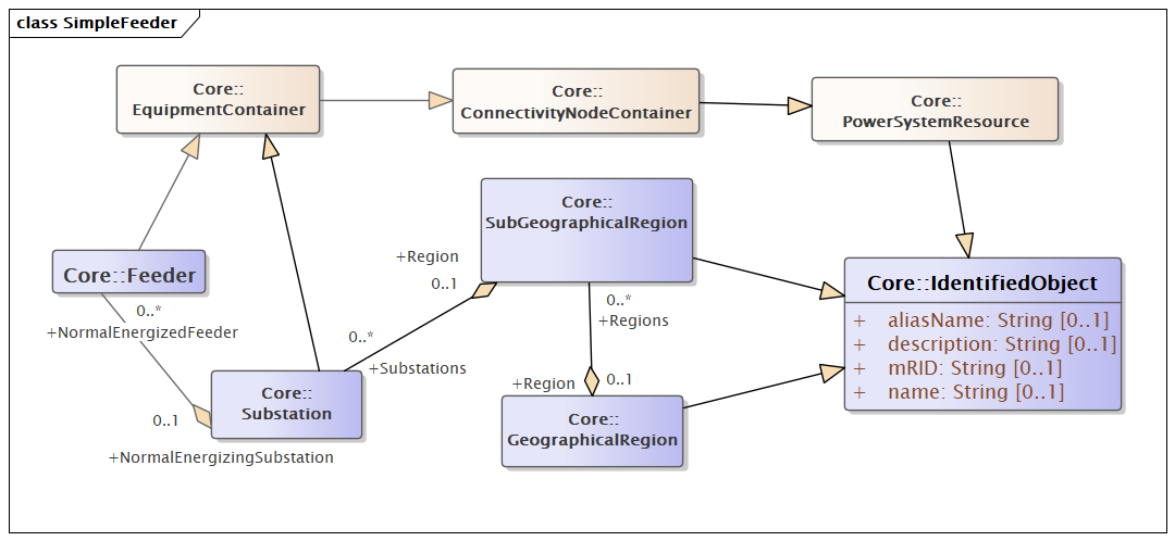
Each kind of triple corresponds to features on the UML diagram. The order of triples in a SPARQL query doesn’t affect the result, although it may affect the run time. With reference to the UML diagram below, the example SPARQL query contents are:

• Lines 2-3 define shorthand prefixes for the RDF and CIM namespaces

• Line 4 selects the name and mRID for a feeder, substation, subregion, and region. The ? refers to temporary variables created in the SPARQL query

• Line 5 selects objects of type c:Feeder, which appears to the left in the UML diagram The matched feeder object(s) will be in variable ?s

• Lines 6 and 7 select the name and mRID attributes for feeder ?s, saving them in temporary variables ?feeder and ?fid, to be returned in Line 4. These attributes are inherited from IdentifiedObject, which appears to the right in the UML diagram. The arrows with triangles indicate inheritance in UML. Note that Feeder also inherits from EquipmentContainer, ConnectivityNodeContainer, and PowerSystemResource before it reaches IdentifiedObject. These three intermediate classes are not of current interest, so they are not highlighted in the UML diagram.

• Line 8 navigates from Feeder to Substation, using the association between them. In the UML diagram, the link with a diamond indicates composition, which is a kind of association. Most associations in CIM are simply lines. An association has cardinality at each end. This one has 0..* at the Feeder end, indicating that a Substation may have zero or more NormalEnergizedFeeders. The cardinality is 0..1 at the Substation end, indicating that a Feeder may have zero or one NormalEnergizingSubstation.

  • A profile of the CIM could be more restrictive, e.g., 1 Feeder.NormalEnergizingSubstation

  • A profile of the CIM could specify when end of the association will be specified. This is usually the end with minimal cardinality, e.g., Feeder.NormalEnergizingSubstation is used but Substation.NormalEnergizedFeeder is not used.

• Lines 9-16 are similar to those already described.

• Line 18 applies optional ordering to the result.

Augmenting the Feeder with Houses

GridLAB-D includes “house models” that represent the behaviors of thermostat-controlled loads and end-use appliances (https://doi.org/10.1109/PES.2011.6039467 and https://doi.org/10.2172/939875). As depicted below, some or all of the metered residential load can be replaced with a house that includes a variety of load components and a second-order equivalent thermal parameter (ETP) model. Heating and cooling loads depend on weather, as does the output of any rooftop solar generation, so the weather can be a correlating factor between household load and generation. Simulations typically run at a time step of 1 to 15 seconds to capture the diversity of load switching times. The GridLAB-D house model has also been used to represent larger buildings, e.g., apartments and strip malls, whenever the assumption of single-zone HVAC system applies. For more complicated building designs, a tool like EnergyPlus should be considered.

With the base CIM XML still in Blazegraph, we will run a script that augments the base case with DER and houses:

• From a command prompt in ./tutorial in the CIMHub repository, invoke python augment123.py

• If everything goes well, you should see two database summaries and two power flow solutions in the output log, completed within several seconds.

• The first listing of class counts in the database represents the base feeder model. There should be 21338 tuples, not including any House, PhotovoltaicUnit, or PowerElectronicsConnection instances.

• There will be a log of adding 287 houses, of different types, into the database. The script will only add houses to secondary service buses, i.e., those with s1 and s2 phasing in CIM. This is a 4-kV feeder; a 15-kV class feeder would have many more houses added.

• The breakdown of house cooling systems is 171 electric, 100 heat pump, and 16 with none. The setpoints and deadbands are randomized. The distributions of these are based on climate region, which is “hot/humid” from the paper.

• There will be a GridLAB-D power flow output, showing about 1761 kW supplied to the feeder. Much of the load has been replaced with houses. At midnight, when the simulation is run by default, the outside temperature is relatively cool and the house cooling systems don’t run. This accounts for the decrease in feeder load, compared to the base case. At midday, house cooling loads will substantially increase the feeder load.

The script augment123.py, reproduced below, does the work with houses and DER. Some of the code is similar to that already describe for base123.py. The significant differences are:

• Line 32 has -h=1 in the export_options. This indicates that GridLAB-D models will be exported with houses to replace split-phase secondary loads.

• Line 33 only asks for the feeder head, L115, in check_branches.

• Lines 42-60 add the houses, export the GridLAB-D model with houses, and run it.

  • Line 43 specifies region 5 for hot/humid

  • Line 43 specifies ieee123_house_uuids.json to store mRID values for houses This file need not exist ahead of time.

  • Line 43 specifies scale=0.4 to reduce the number of houses generated. There are default values assumed for VA/square foot, but in this case, the scale was adjusted to approximately match the base-case peak load without houses.

  • Line 51 copies a default set of end-use appliance schedules to the GridLAB-D model and output directory. These contain time-of-day schedules for a variety of appliances, plug loads, and thermostat-controlled loads. They ship with GridLAB-D.

  • Lines 58-60 show how to write just the tabulated GridLAB-D check_branches output. We don’t want the comparison to the OpenDSS base case, because it does not have houses.

# Copyright (C) 2022 Battelle Memorial Institute
# file: augment123.py

import cimhub.api as cimhub
import cimhub.CIMHubConfig as CIMHubConfig
import subprocess
import stat
import shutil
import os
import sys
import json

cases = [
  {'dssname':'ieee123', 'root':'ieee123houses', 'mRID':'CBE09B55-091B-4BB0-95DA-392237B12640',
   'substation':'Fictitious', 'region':'Texas', 'subregion':'Austin', 'skip_gld': False,
   'glmvsrc': 2401.78, 'bases':[4160.0], 'export_options':' -l=1.0 -p=1.0 -h=1 -a=1 -e=carson',
   'check_branches':[{'dss_link': 'LINE.L115', 'dss_bus': '149', 'gld_link': 'LINE_L115', 'gld_bus': '149'}]},
]

cfg_json = '../queries/cimhubconfig.json'

if sys.platform == 'win32':
  shfile_export = '_export.bat'
  shfile_glm = '_checkglm.bat'
else:
  shfile_export = '_export.sh'
  shfile_glm = '_checkglm.sh'

if __name__ == '__main__':
  CIMHubConfig.ConfigFromJsonFile (cfg_json)

  fp = open('cases.json')
  cases = json.load(fp)
  fp.close()

  mRID = cases[0]['mRID']
  cases[0]['outpath_dss'] = ''

  cimhub.list_feeders ()
  cimhub.summarize_db ()

  # run insert houses, GridLAB-D power flow with houses
  cimhub.insert_houses (mRID=mRID, region=5, seed=0, uuidfile='ieee123_house_uuids.json', scale=0.4)

  cases[0]['root'] = 'ieee123houses'
  cases[0]['export_options'] = ' -l=1.0 -p=1.0 -h=1 -a=1 -e=carson'
  cimhub.make_export_script (cases=cases, scriptname=shfile_export, bClearOutput=False)
  p1 = subprocess.call (shfile_export, shell=True)

  shutil.copyfile('../support/appliance_schedules.glm', './glm/appliance_schedules.glm')
  cimhub.make_glmrun_script (cases=cases, scriptname=shfile_glm, bHouses=True, bProfiles=False)
  p1 = subprocess.call (shfile_glm)
  cimhub.write_glm_flows (glmpath='glm/', rootname=cases[0]['root'],
                          voltagebases=cases[0]['bases'],
                          check_branches=cases[0]['check_branches'])

  # insert aggregated residential rooftop PV, run GridLAB-D with houses and PV
  cimhub.insert_der ('ieee123_der.dat')
  cases[0]['root'] = 'ieee123houseder'

  cimhub.make_export_script (cases=cases, scriptname=shfile_export, bClearOutput=False)
  p1 = subprocess.call (shfile_export, shell=True)

  cimhub.make_glmrun_script (cases=cases, scriptname=shfile_glm, bHouses=True, bProfiles=False)
  p1 = subprocess.call (shfile_glm)
  cimhub.write_glm_flows (glmpath='glm/', rootname=cases[0]['root'], 
                          voltagebases=cases[0]['bases'], 
                          check_branches=cases[0]['check_branches'])

  #insert the player file references for spot loads, run GridLAB-D with houses, PV, variable spot loads
  cimhub.insert_profiles ('oedi_profiles.dat')
  cases[0]['root'] = 'ieee123ecp'

  cimhub.make_export_script (cases=cases, scriptname=shfile_export, bClearOutput=False)
  p1 = subprocess.call (shfile_export, shell=True)

  shutil.copyfile('../support/commercial_schedules.glm', './glm/commercial_schedules.glm')
  cimhub.make_glmrun_script (cases=cases, scriptname=shfile_glm, bHouses=True, bProfiles=True)
  p1 = subprocess.call (shfile_glm)
  cimhub.write_glm_flows (glmpath='glm/', rootname=cases[0]['root'], 
                          voltagebases=cases[0]['bases'], 
                          check_branches=cases[0]['check_branches'])

  # count the elements in the database; should have 287 Houses, 
  # 14 PhotovoltaicUnits, 14 PowerElectronicsConnections
  # 1 EnergyConnectionProfile
  cimhub.summarize_db (cfg_json)

We pick up the discussion of augment123.py in the next section.

Augmenting the Feeder with DER

Continuing with augment123.py:

• Lines 62-65 add DER to the model, which still has houses.

• Lines 67-82 export the GridLAB-D model with houses and DER, run it, and summarize the feeder power. The export_option of -h=1 still applies, but now DER will be exported along with houses. The script still copies appliance schedules to ./glm/.

The file used to insert DER is shown below. Given a base feeder model, we need to know the types, sizes, and bus locations for DER to be inserted. This tutorial inserts 14 single-phase PV DER, representing aggregated residential rooftop solar.

• Line 1 is a file to keep track of mRIDs for the inverters, batteries, panels, and other components inserted. This file does not have to exist beforehand.

• Line 2 specifies the feeder mRID to receive the DER. Even though we only have one feeder in the tutorial, a correct value is still required.

• Lines 3-9 begin with // to indicate comments, which describe the comma- separated fields in subsequent lines

• Lines 10-23 specify one DER per line

  • Field 1 is the DER name

  • Field 2 is the bus name, which is a number in this example. It must already exist in the base feeder model.

  • Field 3 is the phase(s). Note that in CIM, a 240-volt split-phase installation should be specified as s1s2

  • Field 4 can be Battery, Photovoltaic, or SynchronousMachine

  • Field 5 is the maximum panel output in kW

  • Field 6 is the inverter rating in kVA. Per IEEE 1547-2018, this should be higher than the panel kW to satisfy reactive power requirements for either category A or category B.

  • Field 7 is the inverter voltage rating in kV. In this case, it’s 2.4 kV line-to-neutral for single-phase inverters on a 4.16-kV system. Three-phase inverter voltage ratings would be 4.16 kV.

  • Fields 8-9 specify the initial real and reactive power outputs, in kW and kVAR.

  • Field 10 is either catA or catB; see IEEE 1547-2018 Clause 5 for background.

  • Field 11 is the voltage control mode. See IEEE 1547-2018 Clause 5 for background, including the default settings. The script inserting DER always uses the applicable default settings from the standard. (These can be changed through CIM messages, OpenDSS commands or function calls, or GridLAB-D file edits, depending on the context.)

    • CQ is constant reactive power

    • PF is constant power factor

    • VV is Volt-Var mode

    • VW is Volt-Watt mode, although VV_VW would be more common

    • WVAR is Watt-Var mode

    • AVR is Volt-Var mode with autonomously adjusting reference voltage

    • VV_VW is the combination of Volt-Var and Volt-Watt, e.g., as used in Hawaii rule 14H

uuid_file,ieee123_der_uuid.dat
feederID,CBE09B55-091B-4BB0-95DA-392237B12640
//
//name,bus,phases(ABCs1s2),type(Battery,Photovoltaic,SynchronousMachine),kwMax,RatedkVA,RatedkV,kW,kVAR
//  kW is taken as maximum real power
//  for Battery,Photovoltaic: append IEEE 1547 category [catA/catB], control mode [CQ,PF,VV,VW,WVAR,AVR,VV_VW]
//  for Battery: append RatedkWH,StoredkWH
// name,bus,phases(ABCs1s2),type(Battery,Photovoltaic,SynchronousMachine),RatedkVA,RatedkV,kW,kVAR,RatedkWH,StoredkWH
//
DG_6,   7,   A, Photovoltaic, 120.0, 124.0, 2.4, 120.0, 0.0, catA, CQ
DG_12,  17,  C, Photovoltaic, 120.0, 124.0, 2.4, 120.0, 0.0, catA, CQ
DG_18,  29,  A, Photovoltaic, 250.0, 260.0, 2.4, 250.0, 0.0, catA, CQ
DG_30,  43,  B, Photovoltaic, 300.0, 310.0, 2.4, 300.0, 0.0, catA, CQ
DG_36,  49,  B, Photovoltaic, 400.0, 415.0, 2.4, 400.0, 0.0, catA, CQ
DG_42,  55,  A, Photovoltaic, 150.0, 155.0, 2.4, 150.0, 0.0, catA, CQ
DG_48,  63,  A, Photovoltaic, 250.0, 260.0, 2.4, 250.0, 0.0, catA, CQ
DG_54,  68,  A, Photovoltaic, 130.0, 135.0, 2.4, 130.0, 0.0, catA, CQ
DG_60,  75,  C, Photovoltaic, 260.0, 270.0, 2.4, 260.0, 0.0, catA, CQ
DG_66,  80,  B, Photovoltaic, 260.0, 270.0, 2.4, 260.0, 0.0, catA, CQ
DG_72,  87,  B, Photovoltaic, 280.0, 290.0, 2.4, 280.0, 0.0, catA, CQ
DG_78,  96,  B, Photovoltaic, 150.0, 155.0, 2.4, 150.0, 0.0, catA, CQ
DG_84,  104, C, Photovoltaic, 300.0, 310.0, 2.4, 300.0, 0.0, catA, CQ
DG_90,  113, A, Photovoltaic, 350.0, 362.0, 2.4, 350.0, 0.0, catA, CQ

Near the middle of the output log, you should observe:

• The second power flow solution shows around -1510 kW at the feeder head, which means the addition of DER caused reverse power flow at the feeder head.

We pick up the discussion of augment123.py in the next section.

Augmenting the Feeder with Spot Load Profiles

There are some spot loads connected to nodes on the feeder primary, which are not represented with Houses. GridLAB-D and OpenDSS each have mechanisms that allow spot loads to fluctuate. In CIM, the extension class EnergyConnectionProfile is used to associate these variations from individual loads (EnergyConsumer) to files on disk, e.g., loadshapes for OpenDSS, schedules and player files for GridLAB-D.

Continuing with augment123.py:

• Lines 84-87 add spot load fluctuations to the model, which still has houses and DER.

• Lines 89-104 export the GridLAB-D model with houses, DER, and EnergyConnectionProfile. The model is run in GridLAB-D, and the feeder output power is summarized. The export_option of -a=1 at line 32 exports the spot load schedules, along with DER and houses. The script copies commercial schedules to ./glm/, which still contains the appliance schedules from before.

The file used to create the EnergyConnectionProfile is shown below.

• Line 1 is a file to keep track of mRIDs for the EnergyConnectionProfiles inserted. This file does not have to exist beforehand.

• Line 2 specifies the feeder mRID to receive the EnergyConnectionProfile. Even though we only have one feeder in the tutorial, a correct value is still required.

• Lines 3-8 begin with // to indicate comments, which describe the comma- separated fields in subsequent lines

• Line 9 specifies one EnergyConnectionProfile per line

  • Field 1 is the EnergyConnectionProfile name

  • Field 2 is the name of an OpenDSS loadshape for the daily attribute of OpenDSS loads.

  • Field 3 is the name of a GridLAB-D schedule applied as the scaling factor on the base_power attribute of GridLAB-D loads.

  • Field 4 is a comma-separated list of EnergyConsumer (load) names that this EnergyConnectionProfile applies to. The user needs to determine these names from knowledge of the feeder model. In this example, the three-phase loads at s65 and s76 are unbalanced, with different values of base_power on each phase. The three-phase loads at s47 and s48 are balanced. There is a single-phase load on s35a. In the exported GridLAB-D model, a scaling factor defined in office_plugs will apply to all the loads in this list.

uuid_file,ieee123_profiles_uuid.dat
feederID,CBE09B55-091B-4BB0-95DA-392237B12640
//
// name,tokenized list of profiles,comma-separated list of loads
//   profile tokens can be dssDaily, gldSchedule
//   last token must be loads=CSV, where CSV is a comma-separated
//     list of EnergyConsumer (load) names
//
Spot,dssDaily=default,gldSchedule=office_plugs,loads=s35a,s47,s48,s65a,s65b,s65c,s76a,s76b,s76c

The office_plugs schedule is available in a file called commercial_schedules.glm, which comes with GridLAB-D. The scaling factor changes hourly. From 0000 hours to 0700 hours and 2100 to 2400 hours on weekdays, the load scaling factor is 0.6866. From 0900 to 1700 hours each weekday, the load scaling factor is 1.4593. The scaling factor is lower on weekends. The tutorial example runs with this schedule because the script copied the schedule file into GridLAB-D’s working directory at line 95 of augment123.py. You may create or obtain other schedules for GridLAB-D outside of CIMHub. To run your models with these external schedules:

• Examine the output from cimhub.make_glm_runscript. For example, lines 95-96 in augment123.py create ./glm/ieee123ecp_run.glm. This is a small file that includes most of the power system network from ./glm/ieee123ecp_base.glm.

• Around lines 26-27 of the run file, insert #include statements as needed to import your custom schedules. You can either reference local copies of the schedules, or specify full path names to a central location.

• The base file should not require modification.

There are more keywords available for EnergyConnectionProfile, but only gldSchedule is used in this tutorial, and only for the spot loads. The OpenDSS model would run using the EnergyConnectionProfile, because OpenDSS comes with a daily load shape called default. To use other loadshapes, the user would need to make them available to the solver with some manual edits to the exported OpenDSS file.

Near the end of the output log, you should observe:

• The third power flow solution shows around -1889 kW at the feeder head, which means the spot load fluctuation caused more reverse power flow at the feeder head. The spot loads don’t reach their peak values until the middle of the day.

• The second database summary should have 25353 tuples, including 287 House, 14 PhotovoltaicUnit (aka panel), and 14 PowerElectonicsConnection (aka inverter), and 1 EnergyConnectionProfile instances. Some of these have ancillary phase, location, and terminal instances, which contribute to the total increase in the number of tuples.

The Role of mRIDs

In a CIM XML file, the objects are uniquely identified with an rdf:about attribute. These are Universally Unique Identifiers, compliant with web standard RFC 4122. The UUIDs can be used to reference other objects in the CIM XML. The IdentifiedObject.mRID is also a UUID that matches rdf:about. CIMHub and some other implementations use these UUIDs as database keys. In contrast, the IdentifiedObject.name is not guaranteed to be unique and would not be suited to serve as a key. For example, in a GridLAB-D model names must be globally unique, e.g., you can’t have a load and overhead_line both named test. In OpenDSS, the name is only required to be unique within a class, so you can have line.test and load.test in the same model. The use of mRID mitigates some of the complexity in naming objects in CIM.

UUIDs can be created programmatically at the time of first use, but then we want to reuse the same ones. If not, model exchanges, test scripts, and applications that use mRID values might constantly break. OpenDSS and the CIMHub scripts do this automatically. In OpenDSS, a TNamedObject class was inserted in the class hierarchy. This class creats UUIDs on demand, writes them to a file on command, and reloads them from a file on command. In this tutorial example, mRID values are persisted as follows:

• ieee123_uuids.dat maintains the base feeder model mRID values; used by OpenDSS

• ieee123_der_uuid.dat maintains the additional DER mRID values; used by the InsertDER Python function

• ieee123_house_uuids.json maintains the additional House mRID values; used by the InsertHouses Python function

• ieee123_profiles_uuid.dat maintains the additional EnergyConnectionProfile mRID values; used by the InsertProfiles Python function

In GridAPPS-D, the InsertMeasurements Python function maintains mRID values, but these are not used in the CIMHub tutorial.

References:

• A Universally Unique Identifier (UUID) URN Namespace, https://datatracker.ietf.org/doc/html/rfc4122

• OpenDSS Tech Note: CIM (IEC 61968/61970) Support, https://github.com/GRIDAPPSD/CIMHub/blob/feature/SETO/opendsscmd/Common_Information_Model.pdf

Impute Data with Houses and DER

At this point, we have an exported GridLAB-D model with houses and DER, and a nominal power flow solution of this model. We’ll use this model to generate a set of imputed data, based on a summer day in Austin that has a cloud-induced reduction in solar output. We don’t need Blazegraph or CIM for these steps, so you can shut down the database engine if desired. The steps to execute are:

• From a command prompt, navigate to ./tutorial in the CIMHub repository.

• Invoke gridlabd climate_run.glm. This takes a few minutes to run a two-day simulation, at 3-second time steps. Nearly 100 comma-separated value (CSV) files will be created.

• Invoke python combine_recorders.py. This takes several minutes to load the CSV files into a Pandas dataframe, and save the 3-second data into an HDF5 file. (Ignore the warnings about time zone format; this will be fixed on https://github.com/gridlab-d/gridlab-d/issues/1363)

• Invoke python plot_hdf5.py. This will create several plots of the 3-second data, as discussed later. It also re-samples the data at 15-minute intervals, and exports that data to aug11slow.hdf5 and aug11slow.csv

Most of the new work appears in climate_run.glm, reproduced below. This is a normal GridLAB-D input file, which was begun from a copy of ./glm/ieee123ecp_run.glm. The significant additions are:

• Lines 1-2 will enforce a time step of 3 seconds, typical of SCADA data rates

• Line 3 makes the output CSV files easier for Pandas to parse

• Lines 8-14 define a two-day simulation period. The first day “warms up” and diversifies the house models. The imputed data then comes from the second day of simulation. We run 1 minute into the third day, so that 15-minute samples will include midnight between the second and third days.

• Lines 27-31 define local weather from a typical meteorological year (TMY) file for Austin, TX. Customized CSV files can also be used to define the local weather. TMY files include altitude, latitude, and longitude of the weather station, which is important to solar output. If using CSV files, the altitude, latitude, and longitude are specifed manually as attributes of the climate object.

• Line 37 points at the unaltered ieee123ecp_base.glm file exported from CIM. It contains the houses, DER, and spot load schedules, along with the base feeder components.

• Line 49 begins the definition of many GridLAB-D recorders for CSV output. Support files make_load_recorders.py and load_xfmrs.dat were used to help define many of these recorders.

#define INTERVAL=3
#set minimum_timestep=3
#set complex_output_format=RECT  // compatible with Python and Pandas
#set relax_naming_rules=1
#set profiler=1
#set warn=0

clock {
	timezone CST+6CDT;
  // run a day to warm up the houses, and a second day for the data to use
  // July 28 is a full-sun day, August 11 has a cloud transient
	starttime '2013-08-10 00:00:00';
	stoptime '2013-08-12 00:01:00'; // make sure end-of-day is output
};

module powerflow {
  solver_method NR;
  line_capacitance TRUE;
};
module climate;
module generators;
module tape;
module reliability {
  report_event_log false;
};

object climate {
  name localWeather;
  tmyfile "../support/TX-Austin_Mueller_Municipal_Ap_Ut.tmy3";
  interpolate QUADRATIC;
};

module residential;
#include "../support/appliance_schedules.glm";
#include "../support/commercial_schedules.glm";
#define VSOURCE=2401.78
#include "glm/ieee123ecp_base.glm";
#ifdef WANT_VI_DUMP
object voltdump {
  filename climate_volt.csv;
  mode POLAR;
};
object currdump {
  filename climate_curr.csv;
  mode POLAR;
};
#endif

// recorders for imputed data
object recorder {
	parent localWeather;
	property temperature,humidity,solar_flux,pressure,wind_speed;
	interval ${INTERVAL};
	file weather.csv;
}

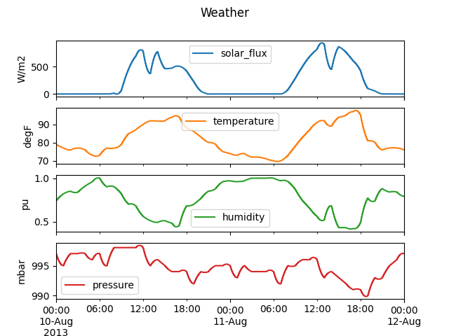
This graph shows the solar irradiance and temperature, along with less important humidity and pressure, over the 2-day simulation period.

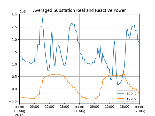
This graph shows real and reactive power at the feeder head. Peak load tends to occur in early evening, i.e., similar to the “duck curve”. At mid-day on both days, there are temporary increases in the net feeder load, caused by transient reductions in solar irradiation. The noise-like variations are caused by appliance and HVAC switching within the house models, and they appear at 3-second sample rates. Fast variations like this appear in real feeder measurements, provided the sample rate is high enough. With more houses on the feeder, the effect is mitigated due to load diversity. On a real feeder, the fast variations are further washed out when the sample rate is 5 minutes or longer. (Note: GridLAB-D doesn’t wash out the variations if we run the house models at longer time steps. Instead, the thermostat loads will switch in concert at the reduced number of time steps. This usually increases the severity of the oscillations.)

This plot shows current magnitudes at the feeder head, with a significant amount of phase unbalance.

This plot separates the house load power (secondaryP), from loads connected to the primary (primaryP) and the DER output (pvP). We can observe that secondaryP is approximately compensated by pvP during much of the day. The primaryP load varies in hourly steps through the two week days according to the office_plugs schedule.

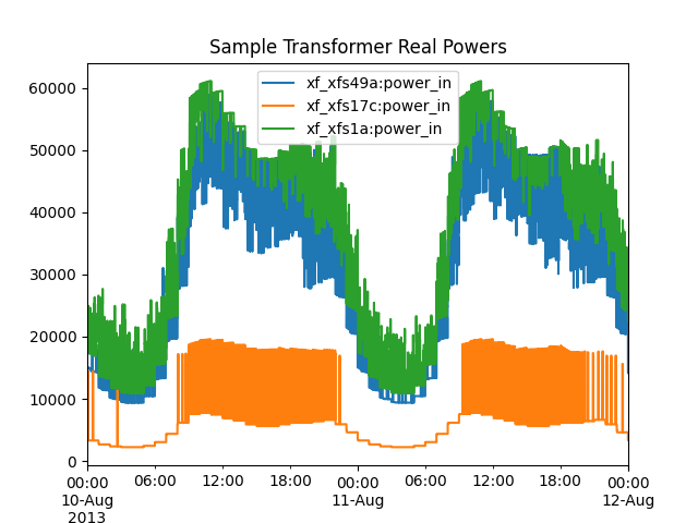
There are 82 transformers that server secondary loads in this model, serving 3.5 houses on average per transformer. This next plot shows the real power for 3 of these transformers. Much of the load switching comes from HVAC, which is especially apparent with xf_xfs17c. All three transformer model loads have more variability than the substation load.

In this plot, the feeder load components have been re-sampled at 15-minute intervals. Variability in secondaryP is much reduced.

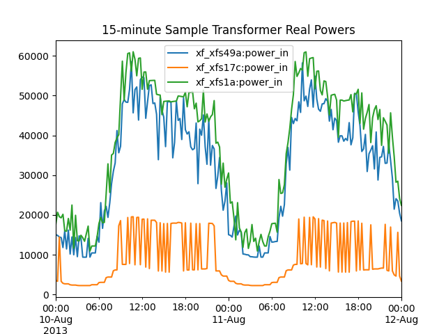
In this plot, the 3 example transformer loads have been re-sampled at 15-minute interevals. This leads to a bias error caused by under-sampling, especially apparent with xf_xfs17c. The bias must exist in secondaryP, but it doesn’t seem so apparent due to aggregation. If we wish to use 15-minute samples down to the transformer level, then a more sophisticated sampling scheme should be considered to remove the bias.

Meter Sampling at 15-Minute Intervals

To create 15-minute average data, without sampling bias, invoke 3sec_data_resample.py. This script applies the pandas functions taking the mean of resample output to create ./15min/aug11avg.csv and ./15min/aug11avg.hdf5 data files. The plot below shows that real and reactive power measured at the substation are now smooth. These graphs may resemble actual utility data sampled at 5 to 60-minute intervals.

In this plot, the rapid on-off switching of HVAC load is also smoothed. The switching still occurs within each 15-minute interval, and it may create voltage fluctuations, but this does not appear in 15-minute interval data.

Creating an Opal-RT (ePHASORSIM) Model

CIMHub can export Opal-RT/ePHASORSIM and Alternative Transient Program (ATP) models.

• The ePHASORSIM.py script in https://github.com/GRIDAPPSD/CIMHub/tree/feature/SETO/CPYDAR shows how to do this with three circuits from the Solar Energy Technologies Office Securing Solar for the Grid (S2G) project. These circuits include:

  • IEEE 13-bus, enhanced with DER

  • IEEE 123-bus, enhanced with DER as in this tutorial

  • EPRI J1 distributed photovoltaic project feeder, which comes with OpenDSS

• ePHASORSIM.py reads SPARQL queries from ./queries/q100.xml

• ePHASORSIM.py should be added to the CIMHub package that is deployed to PyPi

• A similar script, makeATP.py, has been created to produce ATP models that impute PMU and transient data for the OEDI project. This script is only available to licensed ATP users.

Starting with a New OpenDSS File

This last section will show how base123.py could be modified to work with your own OpenDSS file. The steps are:

• First, you start with an OpenDSS file. You should know which buses and branches are important to check, and what the voltage bases are. To illustrate, we will import from ../example/IEEE13_Assets.dss, which is available if you cloned the repository from GitHub. This example file represents one you might create or obtain elsewhere. It’s a version of the IEEE 13-bus system that uses wire spacings and transformer codes to define component impedances. The voltage bases are different, and we need to use a different feeder mRID.

• Second, make a copy of base123.py, and call it test_new.py. Most of this file can be used without changes.

• Third, you need to make a new feeder mRID value. The code at line 26 does this, and we will just use the sample result from line 27.

• Fourth, you need to modify the cases at lines 30-39. In the example below:

  • the new mRID value has been copied from line 27

  • the path to a different OpenDSS file has been provided as dssname

  • the name for exported files has been provided as root

  • skip_gld has been set to True for illustration, even though GridLAB-D will solve this case

  • the new values for substation, region, and subregion are cosmetic for this case

  • new bases match voltage bases in the 13-bus test case

  • the check_branches have been updated for two illustrative locations in the 13-bus test case

cases = [
  {'dssname':'../example/IEEE13_Assets', 'root':'test_new', 'mRID':'CA7CB1B6-BD68-44BF-8C6C-66BB4FA0081D',
   'substation':'Fictitious', 'region':'Massachusetts', 'subregion':'Cambridge', 'skip_gld': True,
   'glmvsrc': 66395.3, 'bases':[480.0, 4160.0, 115000.0], 'export_options':' -l=1.0 -p=1.0 -e=carson',
   'check_branches':[{'dss_link': 'TRANSFORMER.XFM1', 'dss_bus': '633'},
                     {'dss_link': 'LINE.670671', 'dss_bus': '670'}]},
]

• Fifth, you need to comment out the uuids import command, around line 53, with two slashes (//) written to cim_test.dss. Because this UUID file does not exist yet, OpenDSS would exit with an error (TODO: modify OpenDSS to ignore this error).

print ('//uuids {:s}_uuids.dat'.format (root.lower()), file=fp)

• Sixth, you may now run python test_new.py. The very last line of your output log should look like this:

test_new Nbus=[41,41,0] Nlink=[64,64,0] MAEv=[ 0.0000,-1.0000] MAEi=[0.0007,-1.0000]

The MAEv and MAEi values are considered to be good enough for OpenDSS. The values for GridLAB-D are -1, because no GridLAB-D model was produced or checked.

If you run python test_new.py again, the uuids command around line 53 should be uncommented. Otherwise, OpenDSS will regenerate random mRID values for everything except the feeder, which would mean the mRID values can not be tracked.

If you have cloned the full repository, there are many other examples to use as starting points.

Starting with a CIM XML File

There are many different CIM versions and profiles, which may not match the CIMHub profile. To see if that’s the case:

• Load your CIM XML file into Blazegraph, through the Web browser

• Try executing some of the SPARQL from queries/queries.txt in the repository, starting with DistFeeder

• If the query returns nothing, there are some general queries at the top of the queries/queries.txt file that will help you identify class names, attributes, and name spaces used in your CIM XML file.

If there is a mismatch between CIMHub’s profile and your CIM XML file, the model exports and other functions won’t work. There are two options for mitigating the mismatch:

• In the src_python and GMDM subdirectories, there are CIMadapter.py and some other scripts used to translate incoming CIM XML files from the GMDM profile to the CIMHub profile. Those two profiles are close, but not identical. By modifying the scripts, you could adapt your incoming CIM XML to fit CIMHub’s profile.

• You could write your own SPARQL queries to work on the incoming CIM XML. Test those in the web browser first, then translate them into a copy of queries/q100.xml. Once you have working SPARQL queries, make a copy of CPYDAR/ePHASORSIM.py, which can read and run SPARQL from a file like queries/q100.xml. You would modify the Python code in this file to process the SPARQL result sets as needed.